
Desktop Survival Guide
by Graham Williams
|
|
DATA MINING
Desktop Survival Guide by Graham Williams |
|
|||
AdaBoost Algorithm |


|
Boosting employs a weak learning algorithm (which we identify as the
learner). Suppose the dataset (data) consists of ![]() entites described using
entites described using ![]() variables (lines 1 and 2 of the meta-code
below). The
variables (lines 1 and 2 of the meta-code
below). The ![]() th variable (i.e., the last variable of each observation) is
assumed to be the classification of the observation. In the algorithm
presented here we denote the training data (an
th variable (i.e., the last variable of each observation) is
assumed to be the classification of the observation. In the algorithm
presented here we denote the training data (an ![]() by
by ![]() matrix) as
matrix) as
![]() (line 3) and the class associated with each observation in the training
data (a vector of length
(line 3) and the class associated with each observation in the training
data (a vector of length ![]() ) as
) as ![]() (line 4). Without loss of
generality we can restrict the class to be either
(line 4). Without loss of
generality we can restrict the class to be either ![]() (perhaps
representing
(perhaps
representing ![]() ) or
) or ![]() (representing
(representing ![]() ). This will simplify
the mathematics. Each observation in the training data is initially
assigned the same weight:
). This will simplify
the mathematics. Each observation in the training data is initially
assigned the same weight:
![]() (line 5).
(line 5).
The weak learner will need to use the weights associated with each observation. This may be handled directly by the learner (e.g., rpart takes an option to specify the Roption[]weights) or else by generating a modified dataset by sampling the original dataset based on the weights.
The first model, ![]() , is built by applying the weak
, is built by applying the weak
![]() to the
to the ![]() with weights
with weights ![]() (line 7).
(line 7).
![]() , predicting either
, predicting either ![]() or
or ![]() , is then used to
identify the set of indicies of misclassified entities (i.e., where
, is then used to
identify the set of indicies of misclassified entities (i.e., where
![]() , denoted as
, denoted as ![]() (line 8). For a
completely accurate model we would have
(line 8). For a
completely accurate model we would have
![]() . Of
course the model is expected to be only slightly better than random so
ms is unlikely to be empty.
. Of
course the model is expected to be only slightly better than random so
ms is unlikely to be empty.
A relative error ![]() for
for ![]() is calculated as the
relative sum of the weights of the misclassified entities (line 9).
This is used to calculate
is calculated as the
relative sum of the weights of the misclassified entities (line 9).
This is used to calculate ![]() (line 10), used, in turn, to
adjust the weights (line 11). All weights could be either decreased or
increased depending on whether the model correctly classifies the
corresponding observation, as proposed
by (). However, this can be
simplified to only increasing the weights of the misclassified
entities, as proposed
by (). These entities
thus become more important.
(line 10), used, in turn, to
adjust the weights (line 11). All weights could be either decreased or
increased depending on whether the model correctly classifies the
corresponding observation, as proposed
by (). However, this can be
simplified to only increasing the weights of the misclassified
entities, as proposed
by (). These entities
thus become more important.
The learning algorithm is then applied to the new weighted ![]() with the
with the ![]() expected to give more focus on the difficult
entities whilst building this next model,
expected to give more focus on the difficult
entities whilst building this next model, ![]() . The weights
are then modified again using the errors from
. The weights
are then modified again using the errors from ![]() . The
model building and weight modification is then repeated until the new
model performs no better than random (i.e., the error is 50% or more:
. The
model building and weight modification is then repeated until the new
model performs no better than random (i.e., the error is 50% or more:
![]() ), or is perfect (i.e., the error rate is 0% and
), or is perfect (i.e., the error rate is 0% and
![]() is empty), or perhaps after a fixed number of iterations.
is empty), or perhaps after a fixed number of iterations.
![$\textstyle \parbox{0.985\textwidth}{\begin{codebox}
\Procname{$\proc{AdaBoost}(...
... = \Sign\bigl(\sum_{j=1}^{T}
\alpha_j \mathcal{M}_j(x)\bigr)$]
\end{codebox}}$](img98.png)
The final model ![]() (line 14) combines the other models
using a weighted sum of the outputs of these other models. The
weights,
(line 14) combines the other models
using a weighted sum of the outputs of these other models. The
weights, ![]() , reflect the accuracy of each of the constituent
models.
, reflect the accuracy of each of the constituent
models.
A simple example can illustrate the process. Suppose the number of
training entities, ![]() , is 10. Each weight,
, is 10. Each weight, ![]() , is thus initially
, is thus initially
![]() (line 5). Imagine the first model,
(line 5). Imagine the first model, ![]() , correctly
classifies the first 6 of the 10 entities (e.g.,
, correctly
classifies the first 6 of the 10 entities (e.g.,
![]() ), so
that
), so
that
![]() . Then
. Then
![]() , and is the weight that will be used to
multiply the results from this model to be added into the overall
model score. The weights
, and is the weight that will be used to
multiply the results from this model to be added into the overall
model score. The weights
![]() then
become
then
become
![]() .
That is, they now have more importance for the next model
build. Suppose now that
.
That is, they now have more importance for the next model
build. Suppose now that ![]() correctly classifies 8 of the
entities (with
correctly classifies 8 of the
entities (with ![]() ), so that
), so that
![]() and
and
![]() . Thus
. Thus
![]() and
and
![]() . Note how record 8 is proving particularly troublesome and so
its weight is now the highest.
. Note how record 8 is proving particularly troublesome and so
its weight is now the highest.
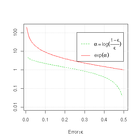
We can understand the behaviour of the function used to weight the
models (
![]() ) and to adjust the observation
weights (
) and to adjust the observation
weights (![]() ) by plotting both of these for the range of
errors we expect (from 0 to 0.5 or 50%).
) by plotting both of these for the range of
errors we expect (from 0 to 0.5 or 50%).
plot(function(x) exp(log((1-x)/x)), xlim=c(0.01, 0.5), ylim=c(0.01, 200),
     xlab=expression(Error: epsilon), ylab="", log="y", lty=1, col=2, yaxt="n")
plot(function(x) log((1-x)/x), add=TRUE, lty=2, col=3)
axis(side=2, at=c(0.01, 0.1, 1, 10, 100), c(0.01, 0.1, 1, 10, 100))
grid()
exp.leg <- expression(alpha == log(over(1-epsilon, epsilon)), exp(alpha))
legend("topright", exp.leg, lty=2:1, col=3:2, inset=c(0.04, 0.1))
|
First, looking at the value of the ![]() 's
(
's
(
![]() ), we see that for errors close to
zero, that is, for very accurate models, the
), we see that for errors close to
zero, that is, for very accurate models, the ![]() (i.e., the
weight that is used to multiply the results from the model) is very
high. For an error of about 5% the multiplier is almost 3, and for a
1% error the multiplier is about 4.6. With an error of approximately
27% (i.e.,
(i.e., the
weight that is used to multiply the results from the model) is very
high. For an error of about 5% the multiplier is almost 3, and for a
1% error the multiplier is about 4.6. With an error of approximately
27% (i.e.,
![]() ) the multiplier is close to 1. For
errors greater than this the model gets weights less than 1, heading
down to a weight of 0 at
) the multiplier is close to 1. For
errors greater than this the model gets weights less than 1, heading
down to a weight of 0 at ![]() .
.
In terms of building the models, the observation weights are multiplied by
![]() . If the model we have just built (
. If the model we have just built (![]() ) is
quite accurate (
) is
quite accurate (![]() close to 0) then fewer entities are being
misclassified, and their weights are increased significantly (e.g.,
for a 5% error the weight is multiplied by 19). For inaccurate models
(as
close to 0) then fewer entities are being
misclassified, and their weights are increased significantly (e.g.,
for a 5% error the weight is multiplied by 19). For inaccurate models
(as ![]() approaches 0.5) the multiplier for the weights
approaches 1. Note that if
approaches 0.5) the multiplier for the weights
approaches 1. Note that if
![]() the multiplier is 1, and
thus no change is made to the weights of the entities. Of course,
building a model on the same dataset with the same weights will build
the same model, thus the criteria for continuing to build a model
tests that
the multiplier is 1, and
thus no change is made to the weights of the entities. Of course,
building a model on the same dataset with the same weights will build
the same model, thus the criteria for continuing to build a model
tests that
![]() .
.